SHAP Integration
MLflow's built-in SHAP integration provides automatic model explanations and feature importance analysis during evaluation. SHAP (SHapley Additive exPlanations) values help you understand what drives your model's predictions, making your ML models more interpretable and trustworthy.
Quick Start: Automatic SHAP Explanations
Enable SHAP explanations during model evaluation with a simple configuration:
import mlflow
import xgboost as xgb
import shap
from sklearn.model_selection import train_test_split
from mlflow.models import infer_signature

# Load the UCI Adult Dataset
X, y = shap.datasets.adult()
X_train, X_test, y_train, y_test = train_test_split(
    X, y, test_size=0.33, random_state=42
)

# Train model
model = xgb.XGBClassifier().fit(X_train, y_train)

# Create evaluation dataset
eval_data = X_test.copy()
eval_data["label"] = y_test

with mlflow.start_run():
    # Log model
    signature = infer_signature(X_test, model.predict(X_test))
    mlflow.sklearn.log_model(model, name="model", signature=signature)
    model_uri = mlflow.get_artifact_uri("model")

    # Evaluate with SHAP explanations enabled
    result = mlflow.evaluate(
        model_uri,
        eval_data,
        targets="label",
        model_type="classifier",
        evaluators=["default"],
        evaluator_config={"log_explainer": True},  # Enable SHAP logging
    )

    print("SHAP artifacts generated:")
    for artifact_name in result.artifacts:
        if "shap" in artifact_name.lower():
            print(f"  - {artifact_name}")
This automatically generates:
- Feature importance plots showing which features matter most
- SHAP summary plots displaying feature impact distributions
- SHAP explainer model saved for future use on new data
- Individual prediction explanations for sample predictions
Understanding SHAP Outputs
Feature Importance Visualization
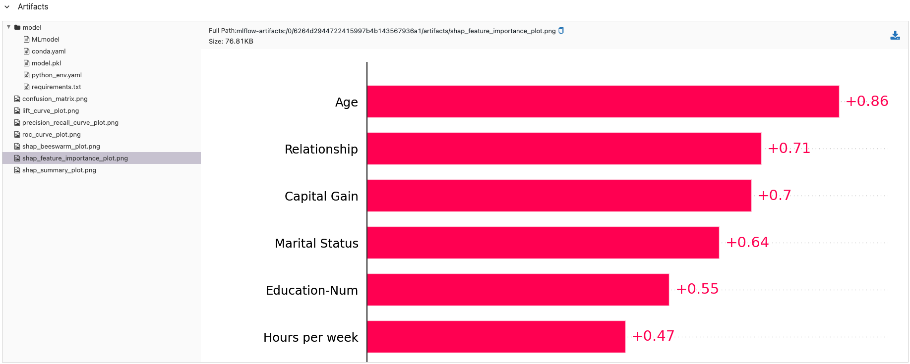
MLflow automatically creates SHAP-based feature importance charts:
# The evaluation generates several SHAP visualizations:
# - shap_feature_importance_plot.png: Bar chart of average feature importance
# - shap_summary_plot.png: Dot plot showing feature impact distribution
# - explainer model: Saved SHAP explainer for generating new explanations

# Access the results
print(f"Model accuracy: {result.metrics['accuracy_score']:.3f}")
print("Generated SHAP artifacts:")
for name, path in result.artifacts.items():
    if "shap" in name:
        print(f"  {name}: {path}")
Configuring SHAP Explanations
Control how SHAP explanations are generated:
# Advanced SHAP configuration
shap_config = {
    "log_explainer": True,  # Save the explainer model
    "explainer_type": "exact",  # Use exact SHAP values (slower but precise)
    "max_error_examples": 100,  # Number of error cases to explain
    "log_model_explanations": True,  # Log individual prediction explanations
}

result = mlflow.evaluate(
    model_uri,
    eval_data,
    targets="label",
    model_type="classifier",
    evaluators=["default"],
    evaluator_config=shap_config,
)
Configuration Options
Explainer Types
"exact": Precise SHAP values using the exact algorithm (slower)"permutation": Permutation-based explanations (faster, approximate)"partition": Tree-based explanations for tree models
Output Control
log_explainer: Whether to save the SHAP explainer as a modelmax_error_examples: Number of misclassified examples to explain in detaillog_model_explanations: Whether to log explanations for individual predictions
Working with SHAP Explainers
- Loading & Using Explainers
- Model Comparison with SHAP
- Custom SHAP Analysis
Once logged, you can load and use SHAP explainers on new data:
# Load the saved SHAP explainer
run_id = "your_run_id_here"
explainer_uri = f"runs:/{run_id}/explainer"

# Load explainer
explainer = mlflow.pyfunc.load_model(explainer_uri)

# Generate explanations for new data
new_data = X_test[:10]  # Example: first 10 samples
explanations = explainer.predict(new_data)

print(f"Generated explanations shape: {explanations.shape}")
print(f"Feature contributions for first prediction: {explanations[0]}")

# The explanations array contains SHAP values for each feature and prediction
Interpreting SHAP Values
def interpret_shap_explanations(explanations, feature_names, sample_idx=0):
    """Interpret SHAP explanations for a specific prediction."""

    sample_explanations = explanations[sample_idx]

    # Sort features by absolute importance
    feature_importance = list(zip(feature_names, sample_explanations))
    feature_importance.sort(key=lambda x: abs(x[1]), reverse=True)

    print(f"SHAP explanation for sample {sample_idx}:")
    print("Top 5 most important features:")

    for i, (feature, importance) in enumerate(feature_importance[:5]):
        direction = "increases" if importance > 0 else "decreases"
        print(f"  {i+1}. {feature}: {importance:.3f} ({direction} prediction)")

    return feature_importance


# Usage
feature_names = X_test.columns.tolist()
top_features = interpret_shap_explanations(explanations, feature_names, sample_idx=0)
Compare feature importance across different models:
from sklearn.ensemble import RandomForestClassifier
from sklearn.linear_model import LogisticRegression


def compare_models_with_shap(models_dict, eval_data, targets):
    """Compare multiple models using SHAP explanations."""

    model_results = {}

    with mlflow.start_run(run_name="Model_Comparison_with_SHAP"):
        for model_name, model in models_dict.items():
            with mlflow.start_run(run_name=f"Model_{model_name}", nested=True):
                # Train model
                model.fit(X_train, y_train)

                # Log model
                signature = infer_signature(X_train, model.predict(X_train))
                mlflow.sklearn.log_model(model, name="model", signature=signature)
                model_uri = mlflow.get_artifact_uri("model")

                # Evaluate with SHAP
                result = mlflow.evaluate(
                    model_uri,
                    eval_data,
                    targets=targets,
                    model_type="classifier",
                    evaluator_config={"log_explainer": True},
                )

                model_results[model_name] = {
                    "accuracy": result.metrics["accuracy_score"],
                    "artifacts": result.artifacts,
                }

                # Tag for easy comparison
                mlflow.set_tag("model_type", model_name)

        # Log comparison summary
        best_model = max(
            model_results.keys(), key=lambda k: model_results[k]["accuracy"]
        )
        mlflow.log_params(
            {"best_model": best_model, "models_compared": len(models_dict)}
        )

    return model_results


# Compare models
models = {
    "random_forest": RandomForestClassifier(n_estimators=100, random_state=42),
    "xgboost": xgb.XGBClassifier(random_state=42),
    "logistic": LogisticRegression(random_state=42),
}

comparison_results = compare_models_with_shap(models, eval_data, "label")

print("Model Comparison Results:")
for model_name, results in comparison_results.items():
    print(f"  {model_name}: {results['accuracy']:.3f} accuracy")
Perform custom SHAP analysis beyond automatic generation:
def custom_shap_analysis(model, data, feature_names):
    """Perform custom SHAP analysis with detailed insights."""

    with mlflow.start_run(run_name="Custom_SHAP_Analysis"):
        # Create SHAP explainer
        explainer = shap.Explainer(model)
        shap_values = explainer(data)

        # Global feature importance
        feature_importance = np.abs(shap_values.values).mean(axis=0)
        importance_dict = dict(zip(feature_names, feature_importance))

        # Log feature importance metrics
        for feature, importance in importance_dict.items():
            mlflow.log_metric(f"importance_{feature}", importance)

        # Create custom visualizations
        import matplotlib.pyplot as plt

        # Summary plot
        plt.figure(figsize=(10, 8))
        shap.summary_plot(shap_values, data, feature_names=feature_names, show=False)
        plt.tight_layout()
        plt.savefig("custom_shap_summary.png", dpi=300, bbox_inches="tight")
        mlflow.log_artifact("custom_shap_summary.png")
        plt.close()

        # Waterfall plot for first prediction
        plt.figure(figsize=(10, 6))
        shap.waterfall_plot(shap_values[0], show=False)
        plt.tight_layout()
        plt.savefig("shap_waterfall_first_prediction.png", dpi=300, bbox_inches="tight")
        mlflow.log_artifact("shap_waterfall_first_prediction.png")
        plt.close()

        # Log analysis summary
        mlflow.log_params(
            {
                "top_feature": max(
                    importance_dict.keys(), key=lambda k: importance_dict[k]
                ),
                "total_features": len(feature_names),
                "samples_analyzed": len(data),
            }
        )

        return shap_values, importance_dict


# Usage
# shap_values, importance = custom_shap_analysis(model, X_test[:100], X_test.columns.tolist())
SHAP Visualization Types
Summary Plots
- Bar plots: Average feature importance across all predictions
- Dot plots: Feature importance distribution showing positive/negative impacts
- Violin plots: Distribution of SHAP values for each feature
Individual Explanations
- Waterfall plots: Step-by-step breakdown of a single prediction
- Force plots: Visual representation of feature contributions
- Decision plots: Path through feature space for predictions
Production SHAP Workflows
- Batch Explanation Generation
- Feature Importance Monitoring
- Performance Optimization
Generate explanations for large datasets efficiently:
def batch_shap_explanations(model_uri, data_path, batch_size=1000):
    """Generate SHAP explanations for large datasets in batches."""

    import pandas as pd

    with mlflow.start_run(run_name="Batch_SHAP_Generation"):
        # Load model and create explainer
        model = mlflow.pyfunc.load_model(model_uri)

        # Process data in batches
        batch_results = []
        total_samples = 0

        for chunk_idx, data_chunk in enumerate(
            pd.read_parquet(data_path, chunksize=batch_size)
        ):
            # Generate explanations for batch
            explanations = generate_explanations(model, data_chunk)

            # Store results
            batch_results.append(
                {
                    "batch_idx": chunk_idx,
                    "explanations": explanations,
                    "sample_count": len(data_chunk),
                }
            )

            total_samples += len(data_chunk)

            # Log progress
            if chunk_idx % 10 == 0:
                print(f"Processed {total_samples} samples...")

        # Log batch processing summary
        mlflow.log_params(
            {
                "total_batches": len(batch_results),
                "total_samples": total_samples,
                "batch_size": batch_size,
            }
        )

        return batch_results


def generate_explanations(model, data):
    """Generate SHAP explanations (placeholder - implement based on your model type)."""
    # This would contain your actual SHAP explanation logic
    # returning mock data for example
    return np.random.random((len(data), data.shape[1]))
Track how feature importance changes over time:
def monitor_feature_importance_drift(current_explainer_uri, historical_importance_path):
    """Monitor changes in feature importance over time."""

    with mlflow.start_run(run_name="Feature_Importance_Monitoring"):
        # Load current explainer
        current_explainer = mlflow.pyfunc.load_model(current_explainer_uri)

        # Generate current explanations
        current_explanations = current_explainer.predict(X_test[:1000])
        current_importance = np.abs(current_explanations).mean(axis=0)

        # Load historical importance (would come from previous runs)
        # historical_importance = load_historical_importance(historical_importance_path)
        # For demo, create mock historical data
        historical_importance = np.random.random(len(current_importance))

        # Calculate importance drift
        importance_drift = np.abs(current_importance - historical_importance)
        relative_drift = importance_drift / (historical_importance + 1e-8)

        # Log drift metrics
        mlflow.log_metrics(
            {
                "max_importance_drift": np.max(importance_drift),
                "avg_importance_drift": np.mean(importance_drift),
                "max_relative_drift": np.max(relative_drift),
                "features_with_high_drift": np.sum(relative_drift > 0.2),
            }
        )

        # Log per-feature drift
        for i, drift in enumerate(importance_drift):
            mlflow.log_metric(f"feature_{i}_drift", drift)

        # Alert if significant drift detected
        high_drift_detected = np.max(relative_drift) > 0.5
        mlflow.log_param("high_drift_alert", high_drift_detected)

        if high_drift_detected:
            print("WARNING: Significant feature importance drift detected!")

        return {
            "current_importance": current_importance,
            "importance_drift": importance_drift,
            "high_drift_detected": high_drift_detected,
        }


# Usage
# drift_results = monitor_feature_importance_drift(
#     "runs:/your_run_id/explainer",
#     "path/to/historical/importance.npy"
# )
Optimize SHAP performance for large-scale applications:
# Optimized configuration for large datasets
def get_optimized_shap_config(dataset_size):
    """Get optimized SHAP configuration based on dataset size."""

    if dataset_size < 1000:
        # Small datasets - use exact methods
        return {
            "log_explainer": True,
            "explainer_type": "exact",
            "max_error_examples": 100,
            "log_model_explanations": True,
        }
    elif dataset_size < 50000:
        # Medium datasets - standard configuration
        return {
            "log_explainer": True,
            "explainer_type": "permutation",
            "max_error_examples": 50,
            "log_model_explanations": True,
        }
    else:
        # Large datasets - optimized for speed
        return {
            "log_explainer": True,
            "explainer_type": "permutation",
            "max_error_examples": 25,
            "log_model_explanations": False,
        }


# Memory-efficient SHAP evaluation
def memory_efficient_shap_evaluation(model_uri, eval_data, targets, sample_size=5000):
    """Perform SHAP evaluation with memory optimization for large datasets."""

    # Sample data if too large
    if len(eval_data) > sample_size:
        sampled_data = eval_data.sample(n=sample_size, random_state=42)
        print(f"Sampled {sample_size} rows from {len(eval_data)} for SHAP analysis")
    else:
        sampled_data = eval_data

    # Get optimized configuration
    config = get_optimized_shap_config(len(sampled_data))

    with mlflow.start_run(run_name="Memory_Efficient_SHAP"):
        result = mlflow.evaluate(
            model_uri,
            sampled_data,
            targets=targets,
            model_type="classifier",
            evaluator_config=config,
        )

        # Log sampling information
        mlflow.log_params(
            {
                "original_dataset_size": len(eval_data),
                "sampled_dataset_size": len(sampled_data),
                "sampling_ratio": len(sampled_data) / len(eval_data),
            }
        )

        return result


# Usage
# result = memory_efficient_shap_evaluation(model_uri, large_eval_data, "target")
Performance Guidelines:
- Small datasets (< 1,000 samples): Use exact SHAP methods for precision
- Medium datasets (1,000 - 50,000 samples): Standard SHAP analysis works well
- Large datasets (50,000+ samples): Consider sampling or approximate methods
- Very large datasets (100,000+ samples): Use batch processing with sampling
Best Practices and Use Cases
When to Use SHAP Integration
SHAP integration provides the most value in these scenarios:
High Interpretability Requirements - Healthcare and medical diagnosis systems, financial services (credit scoring, loan approval), legal and compliance applications, hiring and HR decision systems, and fraud detection and risk assessment.
Complex Model Types - XGBoost, Random Forest, and other ensemble methods, neural networks and deep learning models, custom ensemble approaches, and any model where feature relationships are non-obvious.
Regulatory and Compliance Needs - Models requiring explainability for regulatory approval, systems where decisions must be justified to stakeholders, applications where bias detection is important, and audit trails requiring detailed decision explanations.
Performance Considerations
Dataset Size Guidelines:
- Small datasets (< 1,000 samples): Use exact SHAP methods for precision
- Medium datasets (1,000 - 50,000 samples): Standard SHAP analysis works well
- Large datasets (50,000+ samples): Consider sampling or approximate methods
- Very large datasets (100,000+ samples): Use batch processing with sampling
Memory Management:
- Process explanations in batches for large datasets
- Use approximate SHAP methods when exact precision isn't required
- Clear intermediate results to manage memory usage
- Consider model-specific optimizations (e.g., TreeExplainer for tree models)
Integration with MLflow Model Registry
SHAP explainers can be stored and versioned alongside your models:
def register_model_with_explainer(model_uri, explainer_uri, model_name):
    """Register both model and explainer in MLflow Model Registry."""

    from mlflow.tracking import MlflowClient

    client = MlflowClient()

    # Register the main model
    model_version = mlflow.register_model(model_uri, model_name)

    # Register the explainer as a separate model
    explainer_name = f"{model_name}_explainer"
    explainer_version = mlflow.register_model(explainer_uri, explainer_name)

    # Add tags to link them
    client.set_model_version_tag(
        model_name, model_version.version, "explainer_model", explainer_name
    )

    client.set_model_version_tag(
        explainer_name, explainer_version.version, "base_model", model_name
    )

    return model_version, explainer_version


# Usage
# model_ver, explainer_ver = register_model_with_explainer(
#     model_uri, explainer_uri, "my_classifier"
# )
Conclusion
MLflow's SHAP integration provides automatic model interpretability without additional setup complexity. By enabling SHAP explanations during evaluation, you gain valuable insights into feature importance and model behavior that are essential for building trustworthy ML systems.
Key benefits include:
- Automatic Generation: SHAP explanations created during standard model evaluation
- Production Ready: Saved explainers can generate explanations for new data
- Visual Insights: Automatic generation of feature importance and summary plots
- Model Comparison: Compare interpretability across different model types
SHAP integration is particularly valuable for regulated industries, high-stakes decisions, and complex models where understanding "why" is as important as "what" the model predicts.