Get Started with Keras 3.0 + MLflow
This tutorial is an end-to-end tutorial on training a MINST classifier with Keras 3.0 and logging results with MLflow. It will demonstrate the use of mlflow.keras.MlflowCallback, and how to subclass it to implement custom logging logic.
Keras is a high-level api that is designed to be simple, flexible, and powerful - allowing everyone from beginners to advanced users to quickly build, train, and evaluate models. Keras 3.0, or Keras Core, is a full rewrite of the Keras codebase that rebases it on top of a modular backend architecture. It makes it possible to run Keras workflows on top of arbitrary frameworks — starting with TensorFlow, JAX, and PyTorch.
Download this NotebookImport Packages / Configure Backend
Keras 3.0 is inherently multi-backend, so you will need to set the backend environment variable before importing the package.
[1]:
import os

# You can use 'tensorflow', 'torch' or 'jax' as backend. Make sure to set the environment variable before importing.
os.environ["KERAS_BACKEND"] = "tensorflow"
[2]:
import keras
import numpy as np

import mlflow
Using TensorFlow backend
Load Dataset
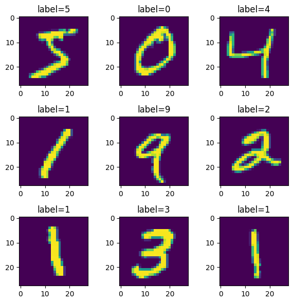
We will use the MNIST dataset. This is a dataset of handwritten digits and will be used for an image classification task. There are 10 classes corresponding to the 10 digits.
[3]:
(x_train, y_train), (x_test, y_test) = keras.datasets.mnist.load_data()
x_train = np.expand_dims(x_train, axis=3)
x_test = np.expand_dims(x_test, axis=3)
x_train[0].shape
[3]:
(28, 28, 1)
[4]:
# Visualize Dataset
import matplotlib.pyplot as plt

grid = 3
fig, axes = plt.subplots(grid, grid, figsize=(6, 6))
for i in range(grid):
    for j in range(grid):
        axes[i][j].imshow(x_train[i * grid + j])
        axes[i][j].set_title(f"label={y_train[i * grid + j]}")
plt.tight_layout()
Build Model
We will use the Keras 3.0 sequential API to build a simple CNN.
[5]:
NUM_CLASSES = 10
INPUT_SHAPE = (28, 28, 1)


def initialize_model():
    return keras.Sequential(
        [
            keras.Input(shape=INPUT_SHAPE),
            keras.layers.Conv2D(32, kernel_size=(3, 3), activation="relu"),
            keras.layers.Conv2D(32, kernel_size=(3, 3), activation="relu"),
            keras.layers.Conv2D(32, kernel_size=(3, 3), activation="relu"),
            keras.layers.GlobalAveragePooling2D(),
            keras.layers.Dense(NUM_CLASSES, activation="softmax"),
        ]
    )


model = initialize_model()
model.summary()
Model: "sequential"
┏━━━━━━━━━━━━━━━━━━━━━━━━━━━━━━━━━┳━━━━━━━━━━━━━━━━━━━━━━━━━━━┳━━━━━━━━━━━━┓
┃ Layer (type)                    ┃ Output Shape              ┃    Param # ┃
┡━━━━━━━━━━━━━━━━━━━━━━━━━━━━━━━━━╇━━━━━━━━━━━━━━━━━━━━━━━━━━━╇━━━━━━━━━━━━┩
│ conv2d (Conv2D)                 │ (None, 26, 26, 32)        │        320 │
├─────────────────────────────────┼───────────────────────────┼────────────┤
│ conv2d_1 (Conv2D)               │ (None, 24, 24, 32)        │      9,248 │
├─────────────────────────────────┼───────────────────────────┼────────────┤
│ conv2d_2 (Conv2D)               │ (None, 22, 22, 32)        │      9,248 │
├─────────────────────────────────┼───────────────────────────┼────────────┤
│ global_average_pooling2d        │ (None, 32)                │          0 │
│ (GlobalAveragePooling2D)        │                           │            │
├─────────────────────────────────┼───────────────────────────┼────────────┤
│ dense (Dense)                   │ (None, 10)                │        330 │
└─────────────────────────────────┴───────────────────────────┴────────────┘
Total params: 19,146 (74.79 KB)
Trainable params: 19,146 (74.79 KB)
Non-trainable params: 0 (0.00 B)
Train Model (Default Callback)
We will fit the model on the dataset, using MLflow’s mlflow.keras.MlflowCallback to log metrics during training.
[6]:
BATCH_SIZE = 64  # adjust this based on the memory of your machine
EPOCHS = 3
Log Per Epoch
An epoch defined as one pass through the entire training dataset.
[7]:
model = initialize_model()

model.compile(
    loss=keras.losses.SparseCategoricalCrossentropy(),
    optimizer=keras.optimizers.Adam(),
    metrics=["accuracy"],
)

run = mlflow.start_run()
model.fit(
    x_train,
    y_train,
    batch_size=BATCH_SIZE,
    epochs=EPOCHS,
    validation_split=0.1,
    callbacks=[mlflow.keras.MlflowCallback(run)],
)
mlflow.end_run()
Epoch 1/3
844/844 ━━━━━━━━━━━━━━━━━━━━ 30s 34ms/step - accuracy: 0.5922 - loss: 1.2862 - val_accuracy: 0.9427 - val_loss: 0.2075
Epoch 2/3
844/844 ━━━━━━━━━━━━━━━━━━━━ 28s 33ms/step - accuracy: 0.9330 - loss: 0.2286 - val_accuracy: 0.9348 - val_loss: 0.2020
Epoch 3/3
844/844 ━━━━━━━━━━━━━━━━━━━━ 28s 33ms/step - accuracy: 0.9499 - loss: 0.1671 - val_accuracy: 0.9558 - val_loss: 0.1491
Log Results
The callback for the run would log parameters, metrics and artifacts to MLflow dashboard.

Log Per Batch
Within each epoch, the training dataset is broken down to batches based on the defined BATCH_SIZE. If we set the callback to not log based on epochs with log_every_epoch=False, and to log every 5 batches with log_every_n_steps=5, we can adjust the logging to be based on the batches.
[8]:
model = initialize_model()

model.compile(
    loss=keras.losses.SparseCategoricalCrossentropy(),
    optimizer=keras.optimizers.Adam(),
    metrics=["accuracy"],
)

with mlflow.start_run() as run:
    model.fit(
        x_train,
        y_train,
        batch_size=BATCH_SIZE,
        epochs=EPOCHS,
        validation_split=0.1,
        callbacks=[mlflow.keras.MlflowCallback(run, log_every_epoch=False, log_every_n_steps=5)],
    )
Epoch 1/3
844/844 ━━━━━━━━━━━━━━━━━━━━ 30s 34ms/step - accuracy: 0.6151 - loss: 1.2100 - val_accuracy: 0.9373 - val_loss: 0.2144
Epoch 2/3
844/844 ━━━━━━━━━━━━━━━━━━━━ 29s 34ms/step - accuracy: 0.9274 - loss: 0.2459 - val_accuracy: 0.9608 - val_loss: 0.1338
Epoch 3/3
844/844 ━━━━━━━━━━━━━━━━━━━━ 28s 34ms/step - accuracy: 0.9477 - loss: 0.1738 - val_accuracy: 0.9577 - val_loss: 0.1454
Log Results
If we log per epoch, we will only have three datapoints, since there are only 3 epochs:

By logging per batch, we can get more datapoints, but they can be noisier:

[9]:
class MlflowCallbackLogPerBatch(mlflow.keras.MlflowCallback):
    def on_batch_end(self, batch, logs=None):
        if self.log_every_n_steps is None or logs is None:
            return
        if (batch + 1) % self.log_every_n_steps == 0:
            self.metrics_logger.record_metrics(logs, self._log_step)
            self._log_step += self.log_every_n_steps
[10]:
model = initialize_model()

model.compile(
    loss=keras.losses.SparseCategoricalCrossentropy(),
    optimizer=keras.optimizers.Adam(),
    metrics=["accuracy"],
)

with mlflow.start_run() as run:
    model.fit(
        x_train,
        y_train,
        batch_size=BATCH_SIZE,
        epochs=EPOCHS,
        validation_split=0.1,
        callbacks=[MlflowCallbackLogPerBatch(run, log_every_epoch=False, log_every_n_steps=5)],
    )
Epoch 1/3
844/844 ━━━━━━━━━━━━━━━━━━━━ 29s 34ms/step - accuracy: 0.5645 - loss: 1.4105 - val_accuracy: 0.9187 - val_loss: 0.2826
Epoch 2/3
844/844 ━━━━━━━━━━━━━━━━━━━━ 29s 34ms/step - accuracy: 0.9257 - loss: 0.2615 - val_accuracy: 0.9602 - val_loss: 0.1368
Epoch 3/3
844/844 ━━━━━━━━━━━━━━━━━━━━ 29s 34ms/step - accuracy: 0.9456 - loss: 0.1800 - val_accuracy: 0.9678 - val_loss: 0.1037