Develop ML model with MLflow and deploy to Kubernetes

Note

This tutorial assumes that you have access to a Kubernetes cluster. However, you can also complete this tutorial on your local machine by using local cluster emulation tools such as Kind or Minikube.

This guide demonstrates how to use MLflow end-to-end for:

• Training a linear regression model with MLflow Tracking.

• Conducting hyper-parameter tuning to find the best model.

• Packaging the model weights and dependencies as an MLflow Model.

• Testing model serving locally with mlserver using the mlflow models serve command.

• Deploying the model to a Kubernetes cluster using KServe with MLflow.

We will cover an end-to-end model development process including model training and testing within this tutorial. If you already have a model and simply want to learn how to deploy it to Kubernetes, you can skip to Step 6 - Test Model Serving Locally

Introduction: Scalable Model Serving with KServe and MLServer

MLflow provides an easy-to-use interface for deploying models within a Flask-based inference server. You can deploy the same inference server to a Kubernetes cluster by containerizing it using the mlflow models build-docker command. However, this approach may not be scalable and could be unsuitable for production use cases. Flask is not designed for high performance and scale (why?), and also manually managing multiple instances of inference servers is backbreaking.

Fortunately, MLflow offers a solution for this. MLflow provides an alternative inference engine that is better suited for larger-scale inference deployments with its support for MLServer, which enables one-step deployment to popular serverless model serving frameworks on Kubernetes, such as KServe, and Seldon Core.

What is KServe?

KServe, formally known as KFServing, provides performant, scalable, and highly-abstracted interfaces for common machine learning frameworks like Tensorflow, XGBoost, scikit-learn, and Pytorch. It offers advanced features that aid in operating large-scale machine learning systems, such as autoscaling, canary rollout, A/B testing, monitoring, explainability, and more, leveraging the Kubernetes ecosystem, including KNative and Istio.

Benefits of using MLflow with KServe

While KServe enables highly scalable and production-ready model serving, deplying your model there might require some effort. MLflow simplifies the process of deploying models to a Kubernetes cluster with KServe and MLServer. Additionally, it offers seamless end-to-end model management as a single place to manage the entire ML lifecycle. This includes experiment tracking, model packaging, versioning, evaluation, and deployment, which we will cover in this tutorial.

Step 1: Installing MLflow and Additional Dependencies

First, please install mlflow to your local machine using the following command:

pip install mlflow[extras]

[extras] will install additional dependencies required for this tutorial including mlserver and scikit-learn. Note that scikit-learn is not required for deployment, just for training the example model used in this tutorial.

You can check if MLflow is installed correctly by running:

mlflow --version

Step 2: Setting Up a Kubernetes Cluster

Kubernetes ClusterLocal Machine Emulation

If you already have access to a Kubernetes cluster, you can install KServe to your cluster by following the official instructions.

Now that you have a Kubernetes cluster running as a deployment target, let’s move on to creating the MLflow Model to deploy.

Step 3: Training the Model

In this tutorial, we will train and deploy a simple regression model that predicts the quality of wine.

Let’s start from training a model with the default hyperparameters. Execute the following code in a notebook or as a Python script.

Note

For the sake of convenience, we use the mlflow.sklearn.autolog() function. This function allows MLflow to automatically log the appropriate set of model parameters and metrics during training. To learn more about the auto-logging feature or how to log manually instead, see the MLflow Tracking documentation.

import mlflow

import numpy as np
from sklearn import datasets, metrics
from sklearn.linear_model import ElasticNet
from sklearn.model_selection import train_test_split


def eval_metrics(pred, actual):
    rmse = np.sqrt(metrics.mean_squared_error(actual, pred))
    mae = metrics.mean_absolute_error(actual, pred)
    r2 = metrics.r2_score(actual, pred)
    return rmse, mae, r2


# Set th experiment name
mlflow.set_experiment("wine-quality")

# Enable auto-logging to MLflow
mlflow.sklearn.autolog()

# Load wine quality dataset
X, y = datasets.load_wine(return_X_y=True)
X_train, X_test, y_train, y_test = train_test_split(X, y, test_size=0.25)

# Start a run and train a model
with mlflow.start_run(run_name="default-params"):
    lr = ElasticNet()
    lr.fit(X_train, y_train)

    y_pred = lr.predict(X_test)
    metrics = eval_metrics(y_pred, y_test)

Now you have trained a model, let’s check if the parameters and metrics are logged correctly, via the MLflow UI. You can start the MLflow UI by running the following command in your terminal:

mlflow ui --port 5000

Then visit http://localhost:5000 to open the UI.

Please open the experient named “wine-quality” on the left, then click the run named “default-params” in the table. For this case, you should see parameters including alpha and l1_ratio and metrics like training_score and mean_absolute_error_X_test.

Step 4: Running Hyperparameter Tuning

Now that we have established a baseline model, let’s attempt to improve its performance by tuning the hyperparameters. We will conduct a random search to identify the optimal combination of alpha and l1_ratio.

from scipy.stats import uniform
from sklearn.model_selection import RandomizedSearchCV

lr = ElasticNet()

# Define distribution to pick parameter values from
distributions = dict(
    alpha=uniform(loc=0, scale=10),  # sample alpha uniformly from [-5.0, 5.0]
    l1_ratio=uniform(),  # sample l1_ratio uniformlyfrom [0, 1.0]
)

# Initialize random search instance
clf = RandomizedSearchCV(
    estimator=lr,
    param_distributions=distributions,
    # Optimize for mean absolute error
    scoring="neg_mean_absolute_error",
    # Use 5-fold cross validation
    cv=5,
    # Try 100 samples. Note that MLflow only logs the top 5 runs.
    n_iter=100,
)

# Start a parent run
with mlflow.start_run(run_name="hyperparameter-tuning"):
    search = clf.fit(X_train, y_train)

    # Evaluate the best model on test dataset
    y_pred = clf.best_estimator_.predict(X_test)
    rmse, mae, r2 = eval_metrics(clf.best_estimator_, y_pred, y_test)
    mlflow.log_metrics(
        {
            "mean_squared_error_X_test": rmse,
            "mean_absolute_error_X_test": mae,
            "r2_score_X_test": r2,
        }
    )

When you reopen the MLflow UI, you should notice that the run “hyperparameter-tuning” contains 5 child runs. MLflow utilizes parent-child relationship, which is particularly useful for grouping a set of runs, such as those in hyper parameter tuning. Here the auto-logging is enabled and MLflow automatically create child runs for the top 5 runs based on the scoring metric, which is negative mean absolute error in this example. You can also create parent and child runs manually, please refer to Create Child Runs for more details.

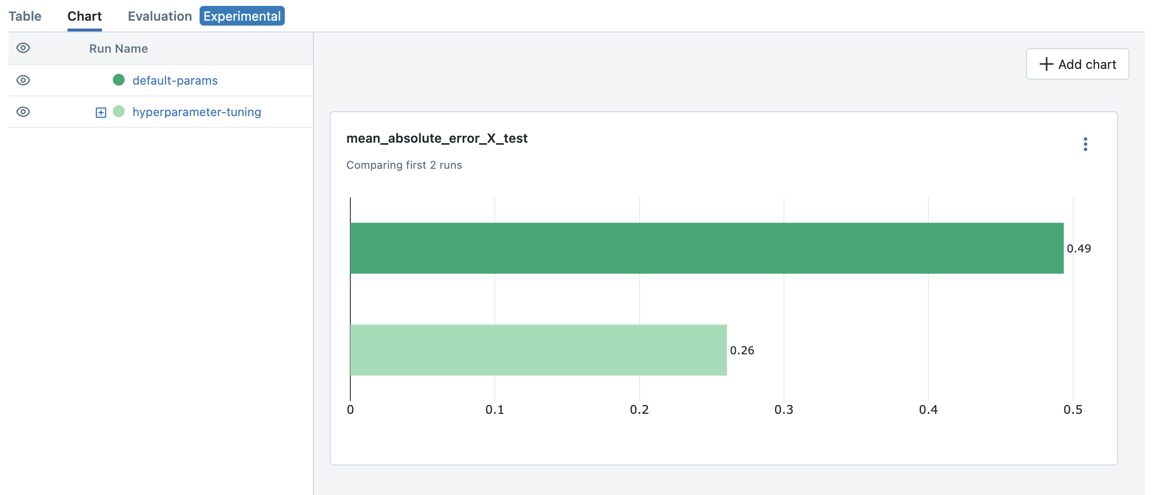
To compare the results and identify the best model, you can utilize the visualization feature in the MLflow UI.

1. Select the first job (“default-params”) and the parent job for hyperparameter tuning (“hyperparameter-turning”).

2. Click on the “Chart” tab to visualize the metrics in a chart.

3. By default, a few bar charts for a predefined set of metrics are displayed.

4. You can add different chart, such as a scatter plot, to compare multiple metrics. For example, we can see the best model from hyperparameter tuning outperforms the default parameter model, in the mean squared error on the test dataset:

You can check the best combination of hyperparameters by looking at the parent run “hyperparameter-tuning”. In this example, the best model was alpha=0.11714084185001972 and l1_ratio=0.3599780644783639 (you may see different results).

Note

To learn more about hyperparameter tuning with MLflow, please refer to Hyperparameter Tuning with MLflow and Optuna.

Step 5: Packaging the Model and Dependencies

Since we are using autologging, MLflow automatically logs the Model for each run. This process conveniently packages the model weight and dependencies in a ready-to-deploy format.

Note

In practice, it is also recommended to use MLflow Model Registry for registering and managing your models.

Let’s take a brief look at how this format appears. You can view the logged model through the Artifacts tab on the Run detail page.

model
├── MLmodel
├── model.pkl
├── conda.yaml
├── python_env.yaml
└── requirements.txt

model.pkl is the file containing the serialized model weight. MLmodel includes general metadata that instructs MLflow on how to load the model. The other files specify the dependencies required to run the model.

Note

If you opt for manual logging, you will need to log the model explicitly using the mlflow.sklearn.log_model function, as shown below:

mlflow.sklearn.log_model(lr, "model")

Step 6: Testing Model Serving Locally

Before deploying the model, let’s first test that the model can be served locally. As outlined in the Deploy MLflow Model Locally, you can run a local inference server with just a single command. Remember to use the enable-mlserver flag, which instructs MLflow to use MLServer as the inference server. This ensures the model runs in the same manner as it would in Kubernetes.

mlflow models serve -m runs:/<run_id_for_your_best_run>/model -p 1234 --enable-mlserver

This command starts a local server listening on port 1234. You can send a request to the server using curl command:

$ curl -X POST -H "Content-Type:application/json" --data '{"inputs": [[14.23, 1.71, 2.43, 15.6, 127.0, 2.8, 3.06, 0.28, 2.29, 5.64, 1.04, 3.92, 1065.0]]' http://127.0.0.1:1234/invocations

{"predictions": [-0.03416275504140387]}

For more information about the request format and response formats, refer to Inference Server Specification.

Step 7: Deploying the Model to KServe

Finally, we are all set to deploy the model to the Kubernetes cluster.

Create Namespace

First, create a test namespace for deploying KServe resources and your model:

kubectl create namespace mlflow-kserve-test

Create Deployment Configuration

Create a YAML file describing the model deployment to KServe.

There are two ways to specify the model for deployment in KServe configuration file:

1. Build a Docker image with the model and specify the image URI.

2. Specify the model URI directly (this only works if your model is stored in remote storage).

Please open the tabs below for details on each approach.

Using Docker ImageUsing Model URI

Register Docker Account

Since KServe cannot resolve a locally built Docker image, you need to push the image to a Docker registry. For this tutorial, we’ll push the image to Docker Hub, but you can use any other Docker registry, such as Amazon ECR or a private registry.

If you don’t have a Docker Hub account yet, create one at https://hub.docker.com/signup.

Build a Docker Image

Build a ready-to-deploy Docker image with the mlflow models build-docker command:

mlflow models build-docker -m runs:/<run_id_for_your_best_run>/model -n <your_dockerhub_user_name>/mlflow-wine-classifier --enable-mlserver

This command builds a Docker image with the model and dependencies, tagging it as mlflow-wine-classifier:latest.

Push the Docker Image

After building the image, push it to Docker Hub (or to another registry using the appropriate command):

docker push <your_dockerhub_user_name>/mlflow-wine-classifier

Write Deployment Configuration

Then create a YAML file like this:

apiVersion: "serving.kserve.io/v1beta1"
kind: "InferenceService"
metadata:
  name: "mlflow-wine-classifier"
  namespace: "mlflow-kserve-test"
spec:
  predictor:
    containers:
      - name: "mlflow-wine-classifier"
        image: "<your_docker_user_name>/mlflow-wine-classifier"
        ports:
          - containerPort: 8080
            protocol: TCP
        env:
          - name: PROTOCOL
            value: "v2"

Deploy Inference Service

Run the following kubectl command to deploy a new InferenceService to your Kubernetes cluster:

$ kubectl apply -f YOUR_CONFIG_FILE.yaml

inferenceservice.serving.kserve.io/mlflow-wine-classifier created

You can check the status of the deployment by running:

$ kubectl get inferenceservice mlflow-wine-classifier

NAME                     URL                                                     READY   PREV   LATEST   PREVROLLEDOUTREVISION   LATESTREADYREVISION
mlflow-wine-classifier   http://mlflow-wine-classifier.mlflow-kserve-test.local   True             100                    mlflow-wine-classifier-100

Note

It may take a few minutes for the deployment status to be ready. For detailed deployment status and logs, run kubectl get inferenceservice mlflow-wine-classifier -oyaml.

Test the Deployment

Once the deployment is ready, you can send a test request to the server.

First, create a JSON file with test data and save it as test-input.json. Ensure the request data is formatted for the V2 Inference Protocol, because we created the model with protocolVersion: v2. The request should look like this:

{
    "inputs": [
      {
        "name": "input",
        "shape": [13],
        "datatype": "FP32",
        "data": [14.23, 1.71, 2.43, 15.6, 127.0, 2.8, 3.06, 0.28, 2.29, 5.64, 1.04, 3.92, 1065.0]
      }
    ]
}

Then send the request to your inference service:

Kubernetes ClusterLocal Machine Emulation

Assuming your cluster is exposed via LoadBalancer, follow these instructions to find the Ingress IP and port. Then send a test request using curl command:

$ SERVICE_HOSTNAME=$(kubectl get inferenceservice mlflow-wine-classifier -n mlflow-kserve-test -o jsonpath='{.status.url}' | cut -d "/" -f 3)
$ curl -v \
  -H "Host: ${SERVICE_HOSTNAME}" \
  -H "Content-Type: application/json" \
  -d @./test-input.json \
  http://${INGRESS_HOST}:${INGRESS_PORT}/v2/models/mlflow-wine-classifier/infer

Troubleshooting

If you have any trouble during deployment, please consult with the KServe official documentation and their MLflow Deployment Guide.

Conclusion

Congratulations on completing the guide! In this tutorial, you have learned how to use MLflow for training a model, running hyperparameter tuning, and deploying the model to Kubernetes cluster.

Further readings:

• MLflow Tracking - Explore more about MLflow Tracking and various ways to manage experiments and models, such as team collaboration.

• MLflow Model Registry - Discover more about MLflow Model Registry for managing model versions and stages in a centralized model store.

• MLflow Deployment - Learn more about MLflow deployment and different deployment targets.

• KServe official documentation - Dive deeper into KServe and its advanced features, including autoscaling, canary rollout, A/B testing, monitoring, explainability, etc.

• Seldon Core official documentation - Learn about Seldon Core, an alternative serverless model serving framework we support for Kubernetes.