Quickstart: Compare runs, choose a model, and deploy it to a REST API

In this quickstart, you will:

• Run a hyperparameter sweep on a training script

• Compare the results of the runs in the MLflow UI

• Choose the best run and register it as a model

• Deploy the model to a REST API

• Build a container image suitable for deployment to a cloud platform

As an ML Engineer or MLOps professional, you can use MLflow to compare, share, and deploy the best models produced by the team. In this quickstart, you will use the MLflow Tracking UI to compare the results of a hyperparameter sweep, choose the best run, and register it as a model. Then, you will deploy the model to a REST API. Finally, you will create a Docker container image suitable for deployment to a cloud platform.

Set up

For a comprehensive guide on getting an MLflow environment setup that will give you options on how to configure MLflow tracking capabilities, you can read the guide here.

Run a hyperparameter sweep

This example tries to optimize the RMSE metric of a Keras deep learning model on a wine quality dataset. It has two hyperparameters that it tries to optimize: learning_rate and momentum. We will use the Hyperopt library to run a hyperparameter sweep across different values of learning_rate and momentum and record the results in MLflow.

Before running the hyperparameter sweep, let’s set the MLFLOW_TRACKING_URI environment variable to the URI of our MLflow tracking server:

export MLFLOW_TRACKING_URI=http://localhost:5000

Note

If you would like to explore the possibilities of other tracking server deployments, including a fully-managed free-of-charge solution with Databricks Community Edition, please see this page.

Import the following packages

import keras
import numpy as np
import pandas as pd
from hyperopt import STATUS_OK, Trials, fmin, hp, tpe
from sklearn.metrics import mean_squared_error
from sklearn.model_selection import train_test_split

import mlflow
from mlflow.models import infer_signature

Now load the dataset and split it into training, validation, and test sets.

# Load dataset
data = pd.read_csv(
    "https://raw.githubusercontent.com/mlflow/mlflow/master/tests/datasets/winequality-white.csv",
    sep=";",
)

# Split the data into training, validation, and test sets
train, test = train_test_split(data, test_size=0.25, random_state=42)
train_x = train.drop(["quality"], axis=1).values
train_y = train[["quality"]].values.ravel()
test_x = test.drop(["quality"], axis=1).values
test_y = test[["quality"]].values.ravel()
train_x, valid_x, train_y, valid_y = train_test_split(
    train_x, train_y, test_size=0.2, random_state=42
)
signature = infer_signature(train_x, train_y)

Then let’s define the model architecture and train the model. The train_model function uses MLflow to track the parameters, results, and model itself of each trial as a child run.

def train_model(params, epochs, train_x, train_y, valid_x, valid_y, test_x, test_y):
    # Define model architecture
    mean = np.mean(train_x, axis=0)
    var = np.var(train_x, axis=0)
    model = keras.Sequential(
        [
            keras.Input([train_x.shape[1]]),
            keras.layers.Normalization(mean=mean, variance=var),
            keras.layers.Dense(64, activation="relu"),
            keras.layers.Dense(1),
        ]
    )

    # Compile model
    model.compile(
        optimizer=keras.optimizers.SGD(
            learning_rate=params["lr"], momentum=params["momentum"]
        ),
        loss="mean_squared_error",
        metrics=[keras.metrics.RootMeanSquaredError()],
    )

    # Train model with MLflow tracking
    with mlflow.start_run(nested=True):
        model.fit(
            train_x,
            train_y,
            validation_data=(valid_x, valid_y),
            epochs=epochs,
            batch_size=64,
        )
        # Evaluate the model
        eval_result = model.evaluate(valid_x, valid_y, batch_size=64)
        eval_rmse = eval_result[1]

        # Log parameters and results
        mlflow.log_params(params)
        mlflow.log_metric("eval_rmse", eval_rmse)

        # Log model
        mlflow.tensorflow.log_model(model, "model", signature=signature)

        return {"loss": eval_rmse, "status": STATUS_OK, "model": model}

The objective function takes in the hyperparameters and returns the results of the train_model function for that set of hyperparameters.

def objective(params):
    # MLflow will track the parameters and results for each run
    result = train_model(
        params,
        epochs=3,
        train_x=train_x,
        train_y=train_y,
        valid_x=valid_x,
        valid_y=valid_y,
        test_x=test_x,
        test_y=test_y,
    )
    return result

Next, we will define the search space for Hyperopt. In this case, we want to try different values of learning-rate and momentum. Hyperopt begins its optimization process by selecting an initial set of hyperparameters, typically chosen at random or based on a specified domain space. This domain space defines the range and distribution of possible values for each hyperparameter. After evaluating the initial set, Hyperopt uses the results to update its probabilistic model, guiding the selection of subsequent hyperparameter sets in a more informed manner, aiming to converge towards the optimal solution.

space = {
    "lr": hp.loguniform("lr", np.log(1e-5), np.log(1e-1)),
    "momentum": hp.uniform("momentum", 0.0, 1.0),
}

Finally, we will run the hyperparameter sweep using Hyperopt, passing in the objective function and search space. Hyperopt will try different hyperparameter combinations and return the results of the best one. We will store the best parameters, model, and evaluation metrics in MLflow.

mlflow.set_experiment("/wine-quality")
with mlflow.start_run():
    # Conduct the hyperparameter search using Hyperopt
    trials = Trials()
    best = fmin(
        fn=objective,
        space=space,
        algo=tpe.suggest,
        max_evals=8,
        trials=trials,
    )

    # Fetch the details of the best run
    best_run = sorted(trials.results, key=lambda x: x["loss"])[0]

    # Log the best parameters, loss, and model
    mlflow.log_params(best)
    mlflow.log_metric("eval_rmse", best_run["loss"])
    mlflow.tensorflow.log_model(best_run["model"], "model", signature=signature)

    # Print out the best parameters and corresponding loss
    print(f"Best parameters: {best}")
    print(f"Best eval rmse: {best_run['loss']}")

Compare the results

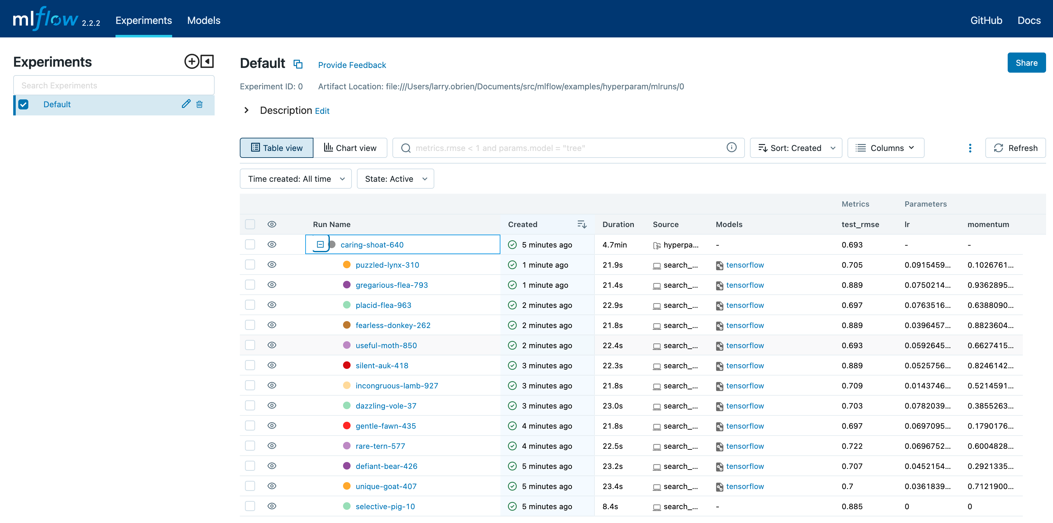
Open the MLflow UI in your browser at the MLFLOW_TRACKING_URI. You should see a nested list of runs. In the default Table view, choose the Columns button and add the Metrics | eval_rmse column and the Parameters | lr and Parameters | momentum column. To sort by RMSE ascending, click the eval_rmse column header. The best run typically has an RMSE on the test dataset of ~0.70. You can see the parameters of the best run in the Parameters column.

Choose Chart view. Choose the Parallel coordinates graph and configure it to show the lr and momentum coordinates and the eval_rmse metric. Each line in this graph represents a run and associates each hyperparameter evaluation run’s parameters to the evaluated error metric for the run.

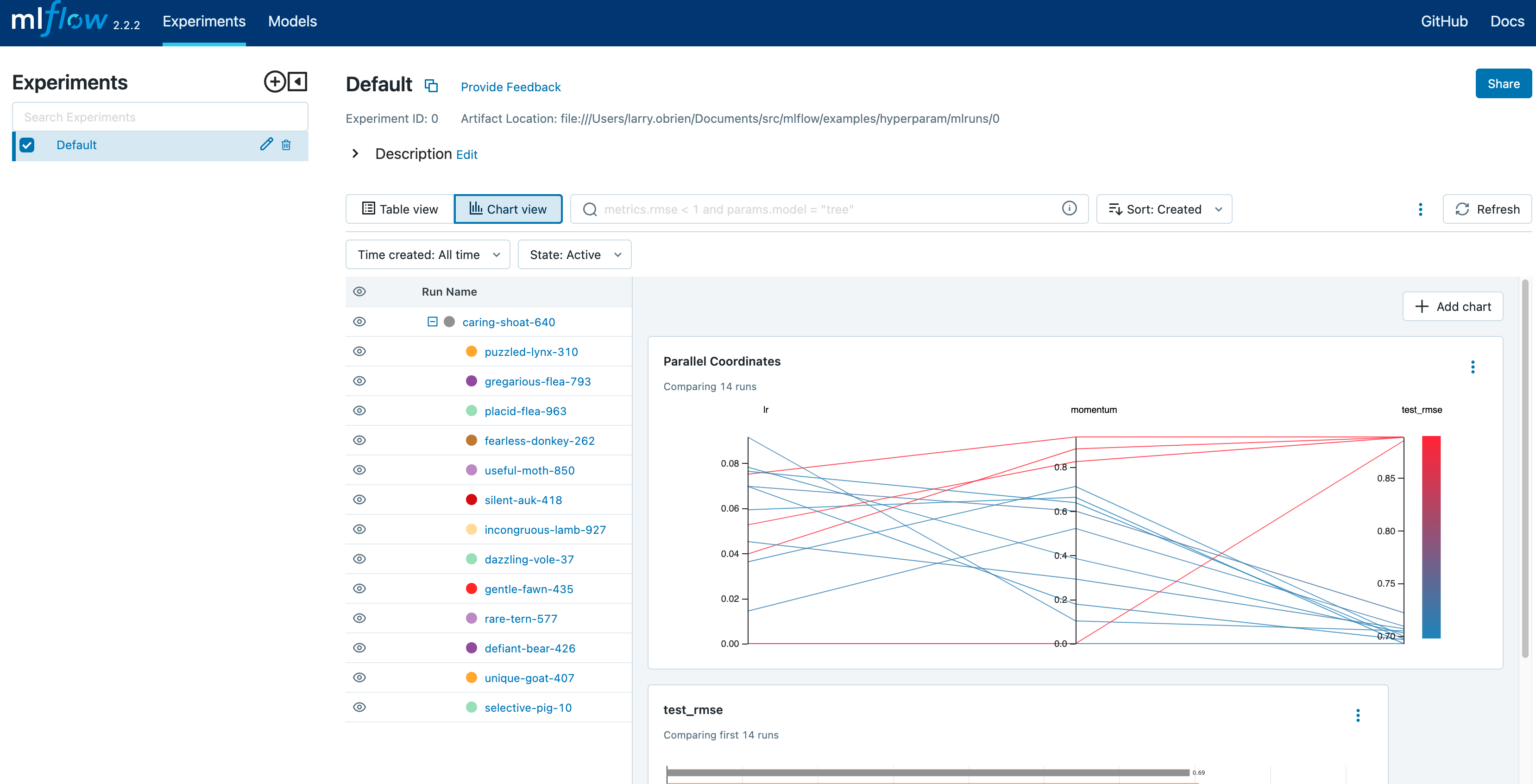
The red graphs on this graph are runs that fared poorly. The lowest one is a baseline run with both lr and momentum set to 0.0. That baseline run has an RMSE of ~0.89. The other red lines show that high momentum can also lead to poor results with this problem and architecture.

The graphs shading towards blue are runs that fared better. Hover your mouse over individual runs to see their details.

Register your best model

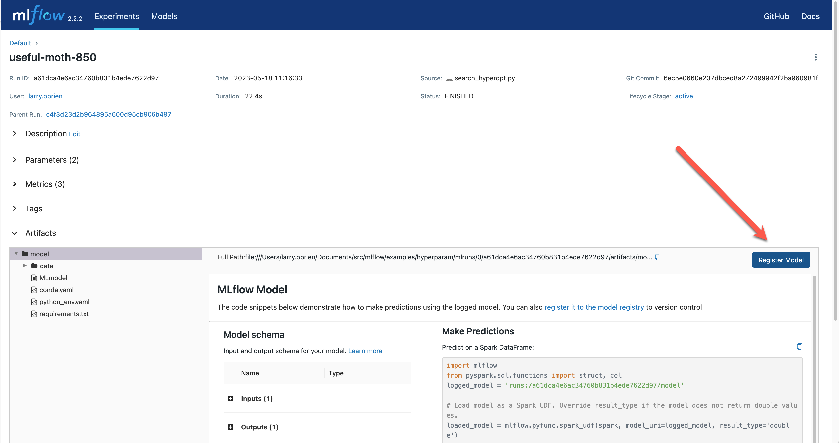
Choose the best run and register it as a model. In the Table view, choose the best run. In the Run Detail page, open the Artifacts section and select the Register Model button. In the Register Model dialog, enter a name for the model, such as wine-quality, and click Register.

Now, your model is available for deployment. You can see it in the Models page of the MLflow UI. Open the page for the model you just registered.

You can add a description for the model, add tags, and easily navigate back to the source run that generated this model. You can also transition the model to different stages. For example, you can transition the model to Staging to indicate that it is ready for testing. You can transition it to Production to indicate that it is ready for deployment.

Transition the model to Staging by choosing the Stage dropdown:

Serve the model locally

MLflow allows you to easily serve models produced by any run or model version. You can serve the model you just registered by running:

mlflow models serve -m "models:/wine-quality/1" --port 5002

(Note that specifying the port as above will be necessary if you are running the tracking server on the same machine at the default port of 5000.)

If the command above is invoked in a new shell session, make sure to re-point tracking server using the export MLFLOW_TRACKING_URI=http://localhost:5000 mentioned above, otherwise MLflow will complain “Registered Model with name=wine-quality not found”

You could also have used a runs:/<run_id> URI to serve a model, or any supported URI described in Artifact Store.

Please note that for production, we do not recommend deploying your model in the same VM as the tracking server because of resource limitation, within this guide we just run everything from the same machine for simplicity.

To test the model, you can send a request to the REST API using the curl command:

curl -d '{"dataframe_split": {
"columns": ["fixed acidity","volatile acidity","citric acid","residual sugar","chlorides","free sulfur dioxide","total sulfur dioxide","density","pH","sulphates","alcohol"],
"data": [[7,0.27,0.36,20.7,0.045,45,170,1.001,3,0.45,8.8]]}}' \
-H 'Content-Type: application/json' -X POST localhost:5002/invocations

Inferencing is done with a JSON POST request to the invocations path on localhost at the specified port. The columns key specifies the names of the columns in the input data. The data value is a list of lists, where each inner list is a row of data. For brevity, the above only requests one prediction of wine quality (on a scale of 3-8). The response is a JSON object with a predictions key that contains a list of predictions, one for each row of data. In this case, the response is:

{"predictions": [{"0": 5.310967445373535}]}

The schema for input and output is available in the MLflow UI in the Artifacts | Model description. The schema is available because the train.py script used the mlflow.infer_signature method and passed the result to the mlflow.log_model method. Passing the signature to the log_model method is highly recommended, as it provides clear error messages if the input request is malformed.

Build a container image for your model

Most routes toward deployment will use a container to package your model, its dependencies, and relevant portions of the runtime environment. You can use MLflow to build a Docker image for your model.

mlflow models build-docker --model-uri "models:/wine-quality/1" --name "qs_mlops"

If the command above erros by

mlflow.exceptions.MlflowException: The configured tracking uri scheme: 'file' is invalid for use with the proxy mlflow-artifact scheme. The allowed tracking schemes are: {'http', 'https'}

This is, again, most likely the tracking server is not pointed at properly (because the command, for example, is run in a seprate shell). Simply run

export MLFLOW_TRACKING_URI=http://localhost:5000

This command builds a Docker image named qs_mlops that contains your model and its dependencies. The model-uri in this case specifies a version number (/1) rather than a lifecycle stage (/staging), but you can use whichever integrates best with your workflow. It will take several minutes to build the image. Once it completes, you can run the image to provide real-time inferencing locally, on-prem, on a bespoke Internet server, or cloud platform. You can run it locally with:

docker run -p 5002:8080 qs_mlops

This Docker run command runs the image you just built and maps port 5002 on your local machine to port 8080 in the container. You can now send requests to the model using the same curl command as before:

curl -d '{"dataframe_split": {"columns": ["fixed acidity","volatile acidity","citric acid","residual sugar","chlorides","free sulfur dioxide","total sulfur dioxide","density","pH","sulphates","alcohol"], "data": [[7,0.27,0.36,20.7,0.045,45,170,1.001,3,0.45,8.8]]}}' -H 'Content-Type: application/json' -X POST localhost:5002/invocations

Running Machine Learning Model NOT Managed by MLflow as REST API in Docker Container

Deploying a trained machine learning model behind a REST API endpoint is an common problem that needs to be solved on the last mile to getting the model into production. The MLflow package provides a flexible abstraction layer that makes deployment via Docker quite easy for those models generated outside of MLflow.

Defining and Storing the Model as a Python Function in MLflow

The model inference logic is wrapped in a class that inherits from PythonModel. There are two functions to implement:

1. load_context() loads the model artifacts

2. predict() runs model inference on the given input and returns the model’s output; the input format will be pandas DataFrame and the output will be a pandas Series of predicted result.

For example

import mlflow.pyfunc
import pandas


class MyModel(mlflow.pyfunc.PythonModel):
    def __init__(self):
        self.model = None

    def load_context(self, context):
        pretrained_model = "my-model"
        this.model = load_model(pretrained_model)

    def predict(self, context, model_input):
        inputs = []
        for _, row in model_input.iterrows():
            inputs.append(row["input_column"])

        return pandas.Series(self.model(inputs))

Next, we save the model locally to a preferred directory. For instance, “my-model-dir/”. We would also need to include a conda environment specifying its dependencies:

conda_env = {
    "channels": ["defaults"],
    "dependencies": [
        "python=3.10.7",
        "pip",
        {
            "pip": ["mlflow", "<other python packages if needed>"],
        },
    ],
    "name": "my_model_env",
}

# Save the MLflow Model
mlflow_pyfunc_model_path = "my-model-dir"
mlflow.pyfunc.save_model(
    path=mlflow_pyfunc_model_path, python_model=MyModel(), conda_env=conda_env
)

In the end, we should have a file called MyModel.py with

import mlflow.pyfunc
import pandas


class MyModel(mlflow.pyfunc.PythonModel):
    def __init__(self):
        self.model = None

    def load_context(self, context):
        pretrained_model = "my-model"
        this.model = load_model(pretrained_model)

    def predict(self, context, model_input):
        inputs = []
        for _, row in model_input.iterrows():
            inputs.append(row["input_column"])

        return pandas.Series(self.model(inputs))


if __name__ == "__main__":
    conda_env = {
        "channels": ["defaults"],
        "dependencies": [
            "python=3.10.7",
            "pip",
            {
                "pip": ["mlflow", "<other python packages if needed>"],
            },
        ],
        "name": "my_model_env",
    }

    # Save the MLflow Model
    mlflow_pyfunc_model_path = "my-model-dir"
    mlflow.pyfunc.save_model(
        path=mlflow_pyfunc_model_path, python_model=MyModel(), conda_env=conda_env
    )

Testing the Model

In case we would like to unit test our model in CI/CD:

loaded_model = mlflow.pyfunc.load_model(mlflow_pyfunc_model_path)

# Evaluate the model
import pandas

test_data = pandas.DataFrame(
    {
        "input_column": ["input1...", "input2...", "input3..."],
        "another_input_column": [...],
    }
)
test_predictions = loaded_model.predict(test_data)
print(test_predictions)

Serving the Model in Docker Container via REST API

build_docker and run container:

mlflow models build-docker --name "my-model-image"

Note

If we see the error of requests.exceptions.ConnectionError: (‘Connection aborted.’, FileNotFoundError(2, ‘No such file or directory’)) from the command above, we can try this workaround:

sudo ln -s "$HOME/.docker/run/docker.sock" /var/run/docker.sock

and then re-run the command

sudo docker run --detach --rm \
  --memory=4000m \
  -p 5001:8080 \
  -v /abs/path/to/my-model-dir:/opt/ml/model \
  -e PYTHONPATH="/opt/ml/model:$PYTHONPATH" \
  -e GUNICORN_CMD_ARGS="--timeout 600 -k gevent --workers=1" \
  "mlflow-model-container"

By the example command above, we

• set the container’s max memory to 4000 megabytes

• set the port forwarding so that the REST API will be accessible at port 5001 on hosting machine

• mount the model directory, i.e. /abs/path/to/my-model-dir, to /opt/ml/model in container

• allow any custom import of modules loaded into /abs/path/to/my-model-dir if our user also put an __init__.py into that directory

• allow long-lasting model inference by setting the internal Flask timeout to be 600 seconds

• set the number of Flask workers to 1

Deploying to a cloud platform

Virtually all cloud platforms allow you to deploy a Docker image. The process varies considerably, so you will have to consult your cloud provider’s documentation for details.

In addition, some cloud providers have built-in support for MLflow. For instance:

• Azure ML

• Databricks

• Amazon SageMaker

• Google Cloud

all support MLflow. Cloud platforms generally support multiple workflows for deployment: command-line, SDK-based, and Web-based. You can use MLflow in any of these workflows, although the details will vary between platforms and versions. Again, you will need to consult your cloud provider’s documentation for details.